Vanishing Gradients Problem Using the ReLU

 Code 1

(.env) [boris@fedora34server NUMPY]$ cat vahish2Issue1.py

# scatter plot of the circles dataset with points colored by class

from sklearn.datasets import make_circles

from numpy import where

from matplotlib import pyplot

# generate circles

X, y = make_circles(n_samples=1000, noise=0.1, random_state=1)

# select indices of points with each class label

for i in range(2):

        samples_ix = where(y == i)

        pyplot.scatter(X[samples_ix, 0], X[samples_ix, 1], label=str(i))

pyplot.legend()

pyplot.show()

****************

Code 2

(.env) [boris@fedora34server NUMPY]$ cat vahish2Issue2.py

# mlp for the two circles classification problem

from sklearn.datasets import make_circles

from sklearn.preprocessing import MinMaxScaler

from keras.layers import Dense

from keras.models import Sequential

from tensorflow.keras.optimizers import SGD

from keras.initializers import RandomUniform

from matplotlib import pyplot

# generate 2d classification dataset

X, y = make_circles(n_samples=1000, noise=0.1, random_state=1)

# scale input data to [-1,1]

scaler = MinMaxScaler(feature_range=(-1, 1))

X = scaler.fit_transform(X)

# split into train and test

n_train = 500

trainX, testX = X[:n_train, :], X[n_train:, :]

trainy, testy = y[:n_train], y[n_train:]

# define model

model = Sequential()

init = RandomUniform(minval=0, maxval=1)

model.add(Dense(5, input_dim=2, activation='tanh', kernel_initializer=init))

model.add(Dense(1, activation='sigmoid', kernel_initializer=init))

# compile model

opt = SGD(learning_rate=0.01, momentum=0.9)

model.compile(loss='binary_crossentropy', optimizer=opt, metrics=['accuracy'])

# fit model

history = model.fit(trainX, trainy, validation_data=(testX, testy), epochs=500, verbose=0)

# evaluate the model

_, train_acc = model.evaluate(trainX, trainy, verbose=0)

_, test_acc = model.evaluate(testX, testy, verbose=0)

print('Train: %.3f, Test: %.3f' % (train_acc, test_acc))

# plot training history

pyplot.plot(history.history['accuracy'], label='train')

pyplot.plot(history.history['val_accuracy'], label='test')

pyplot.legend()

pyplot.show()

*****************

Code 3

(.env) [boris@fedora34server NUMPY]$ cat vahish2Issue3.py

# deeper mlp for the two circles classification problem

from sklearn.datasets import make_circles

from sklearn.preprocessing import MinMaxScaler

from keras.layers import Dense

from keras.models import Sequential

from tensorflow.keras.optimizers import SGD

from keras.initializers import RandomUniform

from matplotlib import pyplot

# generate 2d classification dataset

X, y = make_circles(n_samples=1000, noise=0.1, random_state=1)

scaler = MinMaxScaler(feature_range=(-1, 1))

X = scaler.fit_transform(X)

# split into train and test

n_train = 500

trainX, testX = X[:n_train, :], X[n_train:, :]

trainy, testy = y[:n_train], y[n_train:]

# define model

init = RandomUniform(minval=0, maxval=1)

model = Sequential()

model.add(Dense(5, input_dim=2, activation='tanh', kernel_initializer=init))

model.add(Dense(5, activation='tanh', kernel_initializer=init))

model.add(Dense(5, activation='tanh', kernel_initializer=init))

model.add(Dense(5, activation='tanh', kernel_initializer=init))

model.add(Dense(5, activation='tanh', kernel_initializer=init))

model.add(Dense(1, activation='sigmoid', kernel_initializer=init))

# compile model

opt = SGD(learning_rate=0.01, momentum=0.9)

model.compile(loss='binary_crossentropy', optimizer=opt, metrics=['accuracy'])

# fit model

history = model.fit(trainX, trainy, validation_data=(testX, testy), epochs=500, verbose=0)

# evaluate the model

_, train_acc = model.evaluate(trainX, trainy, verbose=0)

_, test_acc = model.evaluate(testX, testy, verbose=0)

print('Train: %.3f, Test: %.3f' % (train_acc, test_acc))

# plot training history

pyplot.plot(history.history['accuracy'], label='train')

pyplot.plot(history.history['val_accuracy'], label='test')

pyplot.legend()

pyplot.show()

**************

Code5

(.env) [boris@fedora34server NUMPY]$ cat vahish2Issue5.py

# deeper mlp with relu for the two circles classification problem

from sklearn.datasets import make_circles

from sklearn.preprocessing import MinMaxScaler

from keras.layers import Dense

from keras.models import Sequential

from tensorflow.keras.optimizers import SGD

from keras.initializers import RandomUniform

from matplotlib import pyplot

# generate 2d classification dataset

X, y = make_circles(n_samples=1000, noise=0.1, random_state=1)

scaler = MinMaxScaler(feature_range=(-1, 1))

X = scaler.fit_transform(X)

# split into train and test

n_train = 500

trainX, testX = X[:n_train, :], X[n_train:, :]

trainy, testy = y[:n_train], y[n_train:]

# define model

model = Sequential()

model.add(Dense(5, input_dim=2, activation='relu', kernel_initializer='he_uniform'))

model.add(Dense(5, activation='relu', kernel_initializer='he_uniform'))

model.add(Dense(5, activation='relu', kernel_initializer='he_uniform'))

model.add(Dense(5, activation='relu', kernel_initializer='he_uniform'))

model.add(Dense(5, activation='relu', kernel_initializer='he_uniform'))

model.add(Dense(1, activation='sigmoid'))

# compile model

opt = SGD(learning_rate=0.01, momentum=0.9)

model.compile(loss='binary_crossentropy', optimizer=opt, metrics=['accuracy'])

# fit model

history = model.fit(trainX, trainy, validation_data=(testX, testy), epochs=500, verbose=0)

# evaluate the model

_, train_acc = model.evaluate(trainX, trainy, verbose=0)

_, test_acc = model.evaluate(testX, testy, verbose=0)

print('Train: %.3f, Test: %.3f' % (train_acc, test_acc))

# plot training history

pyplot.plot(history.history['accuracy'], label='train')

pyplot.plot(history.history['val_accuracy'], label='test')

pyplot.legend()

pyplot.show()

****************

Code 6

(.env) [boris@fedora34server NUMPY]$ cat vahish2Issue10.py

# deeper mlp with relu for the two circles classification problem with callback

from sklearn.datasets import make_circles

from sklearn.preprocessing import MinMaxScaler

from keras.layers import Dense

from keras.models import Sequential

from tensorflow.keras.optimizers import SGD

from keras.callbacks import TensorBoard

# generate 2d classification dataset

X, y = make_circles(n_samples=1000, noise=0.1, random_state=1)

scaler = MinMaxScaler(feature_range=(-1, 1))

X = scaler.fit_transform(X)

# split into train and test

n_train = 500

trainX, testX = X[:n_train, :], X[n_train:, :]

trainy, testy = y[:n_train], y[n_train:]

# define model

model = Sequential()

model.add(Dense(5, input_dim=2, activation='relu', kernel_initializer='he_uniform'))

model.add(Dense(5, activation='relu', kernel_initializer='he_uniform'))

model.add(Dense(5, activation='relu', kernel_initializer='he_uniform'))

model.add(Dense(5, activation='relu', kernel_initializer='he_uniform'))

model.add(Dense(5, activation='relu', kernel_initializer='he_uniform'))

model.add(Dense(1, activation='sigmoid'))

# compile model

opt = SGD(learning_rate=0.01, momentum=0.9)

model.compile(loss='binary_crossentropy', optimizer=opt, metrics=['accuracy'])

# prepare callback

tb = TensorBoard(histogram_freq=1, write_grads=True)

# fit model

model.fit(trainX, trainy, validation_data=(testX, testy), epochs=500, verbose=0, callbacks=[tb])

***********

Как подавить сообщения Пайтон о том , что при наличии GPU производительность может выше за счет AVX2 FMA директивы :-

"This TensorFlow binary is optimized with oneAPI Deep Neural Network Library (oneDNN) to use the following CPU instructions in performance-critical operations: AVX2 FMA"

Добавьте импорт

import os

os.environ['TF_CPP_MIN_LOG_LEVEL'] = '3'

и выполните

$ export TF_CPP_MIN_LOG_LEVEL=2

Run Code 5 

Run Code 6 above

References

https://machinelearningmastery.com/how-to-fix-vanishing-gradients-using-the-rectified-linear-activation-function/

Uploading в цикле Pandas DataFrames в таблицу встроенной базы данных SQLite3 on Python

 Пример кода и выполнения

(.env) [boris@fedora34server PDSQLITE]$ cat YQDatFrms.py

import numpy as np                                                                   

import pandas as pd                                                                  

from datetime import datetime                                                        

import sqlite3                                                                       

conn = sqlite3.connect('flight.db')                                                  

curs = conn.cursor()                                                                 

curs.execute("create table daily_flights (id integer,  \                           departure date, arrival date, number text, route_id integer)") 

conn.commit()                                                                        

for j in range(1,12):                                                                

   df = pd.DataFrame([[j, datetime(2021, j, j+1, 3+j,10) , \               

      datetime(2021, j, j+1, 5+j,15), chr(64+j)+'1', 3*j+2]], \             

           columns=["id", "departure", "arrival", "number",   \

        "route_id"])                   

   df.to_sql("daily_flights", conn, if_exists="append",index = False)                

data = pd.read_sql_query("select * from daily_flights", conn)

print(data)

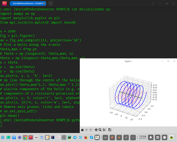
Python depicting a helix via matplotlib and numpy

import numpy as np

import matplotlib.pyplot as plt

from mpl_toolkits.mplot3d import Axes3D

n = 1000

fig = plt.figure()

ax = fig.add_subplot(111, projection='3d')

# Plot a helix along the x-axis

theta_max = 6*np.pi

# theta = np.linspace(0, theta_max, n)

theta = np.linspace(-theta_max,theta_max, n)

x = theta

z =  np.sin(theta)

y =  np.cos(theta)

ax.plot(x, y, z, 'b', lw=2)

# An line through the centre of the helix

ax.plot((-theta_max*1.2, theta_max * 1.2), (0,0), (0,0), color='g', lw=2)

# sin/cos components of the helix (e.g. electric and magnetic field

# components of a circularly-polarized electromagnetic wave

ax.plot(x, y, 0, color='r', lw=1, alpha=0.5)

ax.plot(x, [0]*n, z, color='m', lw=1, alpha=0.5)

# Remove axis planes, ticks and labels

# ax.set_axis_off()

plt.show()

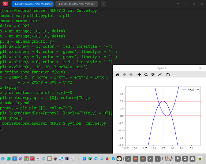
Решение задачи 17 371 Вариант Ларина с помощью Python (numpy,matplotlib)

 Текст задачи

==============

Python code

==============

import matplotlib.pyplot as plt

import numpy as np

delta = 0.025

x = np.arange(-10, 10, delta)

y = np.arange(-10, 10, delta)

p, q = np.meshgrid(x, y)

plt.axhline(y = 5, color = 'red', linestyle = '-')

plt.axhline(y = 4, color = 'green', linestyle = '-')

plt.axhline(y = 1, color = 'green', linestyle = '-')

plt.axhline(y = 0, color = 'red', linestyle = '-')

plt.axvline(0, -10, 10, label='y axis')

# define some function f(x,y)

f = lambda x, y: x**4 - 2*x**3 - 4*x**2 + 10*x \

        - 5 - 2*x*y + 6*y - y**2

z=f(p,q)

# plot contour line of f(x,y)==0

plt.contour(p, q, z , [0], colors=["b"])

# make legend

proxy, = plt.plot([], color="b")

plt.legend(handles=[proxy], labels=["f(x,y) = 0"])

plt.show()

Из плота нетрудно видеть при каких а горизонтальные линии имеют не более 3-ех точек пересения с графиком.

Ответ : а ∈ (-infinity ; 0] ∪ {1;4}∪[5 ; +infinity)

Метрики для оценки алгоритмов машинного обучения в Python

 (.env) [boris@fedora34server YANDEXQ]$ cat predict.py

import pandas

from sklearn import model_selection

from sklearn.linear_model import LogisticRegression

from sklearn.metrics import classification_report

url = "https://raw.githubusercontent.com/jbrownlee/Datasets/master/pima-indians-diabetes.data.csv"

names = ['preg', 'plas', 'pres', 'skin', 'test', 'mass', 'pedi', 'age', 'class']

dataframe = pandas.read_csv(url, names=names)

array = dataframe.values

X = array[:,0:8]

Y = array[:,8]

test_size = 0.33

seed = 7

X_train, X_test, Y_train, Y_test = model_selection.train_test_split(X, Y, test_size=test_size, random_state=seed)

model = LogisticRegression(solver='lbfgs', max_iter=120)

model.fit(X_train, Y_train)

predicted = model.predict(X_test)

report = classification_report(Y_test, predicted)

print(report)

(.env) [boris@fedora34server YANDEXQ]$ python predict.py

              precision    recall  f1-score   support

         0.0       0.81      0.88      0.84       162

         1.0       0.74      0.63      0.68        92

    accuracy                           0.79       254

   macro avg       0.78      0.75      0.76       254

weighted avg       0.78      0.79      0.78       254

(.env) [boris@fedora34server YANDEXQ]$ cat regres01.py

import pandas

from sklearn import model_selection

from sklearn.linear_model import LinearRegression

url = "https://raw.githubusercontent.com/jbrownlee/Datasets/master/housing.data"

names = ['CRIM', 'ZN', 'INDUS', 'CHAS', 'NOX', 'RM', 'AGE', 'DIS', 'RAD', 'TAX', 'PTRATIO', 'B', 'LSTAT', 'MEDV']

dataframe = pandas.read_csv(url, delim_whitespace=True, names=names)

array = dataframe.values

X = array[:,0:13]

Y = array[:,13]

seed = 7

kfold = \ model_selection.KFold(n_splits=10,shuffle=True,random_state=seed)

model = LinearRegression()

scoring = 'neg_mean_absolute_error'

results = model_selection.cross_val_score(model, X, Y, cv=kfold, scoring=scoring)

print(("MAE: %.3f (%.3f)") % (results.mean(), results.std()))

(.env) [boris@fedora34server YANDEXQ]$ python regres01.py

MAE: -3.387 (0.667)

(.env) [boris@fedora34server YANDEXQ]$ cat regres02.py

# Cross Validation Regression MSE

import pandas

from sklearn import model_selection

from sklearn.linear_model import LinearRegression

url = "https://raw.githubusercontent.com/jbrownlee/Datasets/master/housing.data"

names = ['CRIM', 'ZN', 'INDUS', 'CHAS', 'NOX', 'RM', 'AGE', 'DIS', 'RAD', 'TAX', 'PTRATIO', 'B', 'LSTAT', 'MEDV']

dataframe = pandas.read_csv(url, delim_whitespace=True, names=names)

array = dataframe.values

X = array[:,0:13]

Y = array[:,13]

seed = 7

kfold = \ model_selection.KFold(n_splits=10,shuffle=True,random_state=seed)

model = LinearRegression()

scoring = 'neg_mean_squared_error'

results = model_selection.cross_val_score(model, X, Y, cv=kfold, scoring=scoring)

print(("MSE: %.3f (%.3f)") % (results.mean(), results.std()))

(.env) [boris@fedora34server YANDEXQ]$ python regres02.py

MSE: -23.747 (11.143)

(.env) [boris@fedora34server YANDEXQ]$ cat regres03.py

import pandas

from sklearn import model_selection

from sklearn.linear_model import LinearRegression

url = "https://raw.githubusercontent.com/jbrownlee/Datasets/master/housing.data"

names = ['CRIM', 'ZN', 'INDUS', 'CHAS', 'NOX', 'RM', 'AGE', 'DIS', 'RAD', 'TAX', 'PTRATIO', 'B', 'LSTAT', 'MEDV']

dataframe = pandas.read_csv(url, delim_whitespace=True, names=names)

array = dataframe.values

X = array[:,0:13]

Y = array[:,13]

seed = 7

kfold    \ =  model_selection.KFold(n_splits=10,shuffle=True,random_state=seed)

model = LinearRegression()

scoring = 'r2'

results = model_selection.cross_val_score(model, X, Y, cv=kfold, scoring=scoring)

print(("R^2: %.3f (%.3f)") % (results.mean(), results.std()))

(.env) [boris@fedora34server YANDEXQ]$ python regres03.py

R^2: 0.718 (0.099)

References

https://machinelearningmastery.com/metrics-evaluate-machine-learning-algorithms-python/

Решение задачи 17 369 Вариант Ларина с помощью Python (numpy,matplotlib,sympy)

Решение с помощью Пайтон, импортируя numpy,matplotlib,sympy в пайтон виртуальное окружение.

Совмещая условие задачи с геометрией плота получаем значения для параметра а = {-2;2; -3*6^(1/2)/4; -3*6^(1/2)/4}. Рассчеты ординат точек экстремума и точек пересечения голубой и красной кривых проделаны стандартными средствами мат. анализа. Plot строит график числителя дроби в аОх плоскости a(x)= x^3/(4-2x^2) и знаменателя dvr(x) = x/(3-x^2). Аналитически находятся корни a'(x) как {-6^(1/2); 6^(1/2} и их ординаты по оси "а" {-3*6^(1/2)/4; 3*6^(1/2)/4}, прямые а=-3*6^(1/2)/4 и а=3*6^(1/2)/4 пересекут график а(х) только в 2-ух точках, а также точки пересечения a(x)=dvr(x) {-1,1,-2,2}. В силу условия задачи нас интересуют ординаты по "a" только {-2,2}. Эти точки лежащие на кривой а(х) вне [-3*6^(1/2)/4; -3*6^(1/2)/4] по оси "a" следует выколоть и тогда а =2 и а =-2 пересекут график а(х) ровно 2-ух точках, а значения их ординат дадут еще два значения а - это {-2,2}, так как в них dvr(x)=a(x) иначе говоря

a(x)=x/(3-x^2) <=> a(x)*(3-x^2)=x <=> a(x)*x^2-3*a(x)+x=0

import matplotlib.pyplot as plt

import numpy as np

from sympy import sympify, lambdify

from sympy.abc import x

fig = plt.figure('a0x - plane')

ax = fig.add_subplot(111)

ax.spines['left'].set_position('zero')

ax.spines['right'].set_color('none')

ax.spines['bottom'].set_position('zero')

ax.spines['top'].set_color('none')

ax.xaxis.set_ticks_position('bottom')

ax.yaxis.set_ticks_position('left')

# setup x and y ranges and precision

xline = np.arange(-5.5,5.5,0.01)

plt.axhline(y = (3*6**(0.5))/4, color = 'green', linestyle = '-')

plt.axhline(y = -(3*6**(0.5))/4, color = 'green', linestyle = '-')

plt.axhline(y =  2.0, color = 'green', linestyle = '-')

plt.axhline(y = -2.0, color = 'green', linestyle = '-')

myfunction=sympify(x**3/(4-2*x**2))

myfunctionDvr=sympify(x/(3-x**2))

mylambdifiedfunction=lambdify(x,myfunction,'numpy')

mylambdifiedfunctionDvr=lambdify(x,myfunctionDvr,'numpy')

ax.plot(xline, mylambdifiedfunction(xline),zorder=100,linewidth=2,color='blue')

ax.plot(xline, mylambdifiedfunctionDvr(xline),zorder=100,linewidth=1,color='red')

ax.set_xbound(-10,10)

ax.set_ybound(-5,5)

plt.show()

Buiding graph via python module importing networkx,plotly

 (.env) [boris@fedora34server NUMPY]$ cat  graphYQ1011.py

import plotly.graph_objects as go

import networkx as nx

G = nx.random_geometric_graph(200, 0.125)

edge_x = []

edge_y = []

for edge in G.edges():

    x0, y0 = G.nodes[edge[0]]['pos']

    x1, y1 = G.nodes[edge[1]]['pos']

    edge_x.append(x0)

    edge_x.append(x1)

    edge_x.append(None)

    edge_y.append(y0)

    edge_y.append(y1)

    edge_y.append(None)

edge_trace = go.Scatter(

    x=edge_x, y=edge_y,

    line=dict(width=0.5, color='#888'),

    hoverinfo='none',

    mode='lines')

node_x = []

node_y = []

for node in G.nodes():

    x, y = G.nodes[node]['pos']

    node_x.append(x)

    node_y.append(y)

node_trace = go.Scatter(

    x=node_x, y=node_y,

    mode='markers',

    hoverinfo='text',

    marker=dict(

        showscale=True,

        # colorscale options

        #'Greys' | 'YlGnBu' | 'Greens' | 'YlOrRd' | 'Bluered' | 'RdBu' |

        #'Reds' | 'Blues' | 'Picnic' | 'Rainbow' | 'Portland' | 'Jet' |

        #'Hot' | 'Blackbody' | 'Earth' | 'Electric' | 'Viridis' |

        colorscale='YlGnBu',

        reversescale=True,

        color=[],

        size=10,

        colorbar=dict(

            thickness=15,

            title='Node Connections',

            xanchor='left',

            titleside='right'

        ),

        line_width=2))

node_adjacencies = []

node_text = []

for node, adjacencies in enumerate(G.adjacency()):

    node_adjacencies.append(len(adjacencies[1]))

    node_text.append('# of connections: '+str(len(adjacencies[1])))

node_trace.marker.color = node_adjacencies

node_trace.text = node_text

fig = go.Figure(data=[edge_trace, node_trace],

             layout=go.Layout(

                title='<br>Network graph made with Python',

                titlefont_size=16,

                showlegend=False,

                hovermode='closest',

                margin=dict(b=20,l=5,r=5,t=40),

                annotations=[ dict(

                    text="Python code: <a href='https://plotly.com/ipython-notebooks/network-graphs/'> https://plotly.com/ipython-notebooks/network-graphs/</a>",

                    showarrow=False,

                    xref="paper", yref="paper",

                    x=0.005, y=-0.002 ) ],

                xaxis=dict(showgrid=False, zeroline=False, showticklabels=False),

                yaxis=dict(showgrid=False, zeroline=False, showticklabels=False))

                )

fig.show()

References

Sunday, December 26, 2021